A (somewhat) gentle introduction to lattice-based post-quantum cryptography

In recent years, significant progress in researching and building quantum computers has been made. A fully-fledged quantum computer would be able to efficiently solve a distinct set of mathematical problems like integer factorization and the discrete logarithm, which are the basis for a wide range of cryptographic schemes. In 2016, NIST announced an open competition with the goal of finding and standardizing suitable algorithms for quantum-resistant cryptography. The standardization effort by NIST is aimed at post-quantum secure KEMs and digital signatures. In this article, two of the to-be-standardized algorithms, Kyber and Dilithium, are presented and some of their mathematical details are outlined. Both algorithms are based on so-called lattices and the thereupon constructed »Learning with Errors«, which we will get to know in the following.

14. June 2023

1. Lattice fundamentals
1.1 Lattices
1.2 Computational lattice problems
1.3 Shortest vector problem
1.4 Closest vector problem
2. LWE fundamentals
2.1 Learning with errors
2.2 Decisional LWE
2.3 Linking LWE to computational lattice problems
2.4 LWE-based encryption schemes
2.5 Flavors of LWE: Ring-LWE and Module-LWE
3. Kyber
4. Dilithium
5. Bibliography

1. Lattice fundamentals

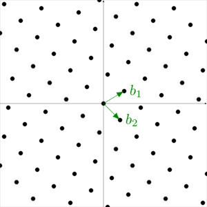
The cryptographic interest in lattices mainly arises from the fact that a given lattice \(L\) can have widely different bases (i.e., different "descriptions" of the lattice). While a good basis can simplify some computational tasks significantly, a bad basis can make them almost impossible. In this section we will give a short introduction to the fundamental mathematics and the two most important computational problems of lattices.

1.1 Lattices

Definition 1.1. (lattice, basis)

Let \(B = \{b_1, b_2, ... , b_m\}\) be a set of linearly independent vectors of \(\mathbb{R}^n\). Then, the set of all integer linear combinations \[ L(B) = \left\{ \sum_i a_ib_i \mid a_i \in \mathbb{Z} \right\} \subset \mathbb{R}^n \] is called \(\textbf{lattice}\) in \( \mathbb{R}^n\) generated by \(B\). We furthermore refer to \(B\) as a \(\textbf{basis}\) of the lattice \( L\).

We can equivalently generate \(L\) via a matrix \(B\) containing the basis vectors as column vectors.

Definition 1.2. (lattice, rank, dimension, full-rank lattice)

Let \(\{b_1, b_2, ... , b_m\}\) be a set of linearly independent vectors of \(\mathbb{R}^n\). Let \(B\) be the \(n \times m\) matrix with column vectors \(b_1, ..., b_m\). Then \[ L(B) = \{Bx \mid x \in \mathbb{Z}^m\} \] is called \(\textbf{lattice}\) in \(\mathbb{R}^n\) generated by \(B\). We call \(m\) the \(\textbf{rank}\) and \(n\) the \(\textbf{dimension}\) of the lattice. For \(m\) equals \(n\), the lattice is called \(\textbf{full-rank lattice}\).

Observe that the basis underlying a lattice \(L\) is not unique. For instance, the lattice generated by the vectors

\( \begin{pmatrix} 0 \\ 1 \end{pmatrix}, \begin{pmatrix} 1 \\ 0 \end{pmatrix} \)

is \(\mathbb{Z}^2\), the set of all integer points. \(\mathbb{Z}^2\) is also generated by the vectors

\( \begin{pmatrix} 2 \\ 1 \end{pmatrix}, \begin{pmatrix} 1 \\ 1 \end{pmatrix} \)

On the other hand, \(n\) linearly independent vectors in \( \mathbb{Z}^n\) are not necessarily a basis of \( \mathbb{Z}^n\). As an example, observe that the modified vectors from the example above

\( \begin{pmatrix} 2 \\ 0 \end{pmatrix}, \begin{pmatrix} 1 \\ 1 \end{pmatrix} \)

do not form a basis of \(\mathbb{Z}^2\).

1.2 Computational lattice problems

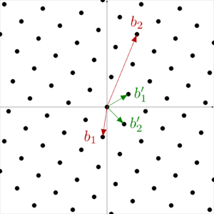
The particular structure of lattices allows them to have special mathematical properties. The following computations can be efficiently evaluated using linear algebra algorithms:

Let \(g_1, ..., g_k \in \mathbb{R}^n\) be a set of vectors generating the lattice \(L\). Calculate a basis \(b_1, ..., b_m \in \mathbb{R}^n\) of \(L\).
Let \(L\) be a lattice. Evaluate whether a given vector \(c\) is an element of \(L\).

Other computational lattice problems appear to be generally hard and are even believed to be resistant against Shor’s algorithm. Therefore, they are interesting candidates for usage in post-quantum-cryptography. These problems are presented in the following.

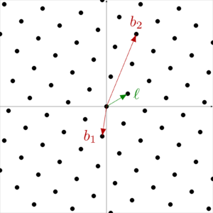
1.3 Shortest vector problem

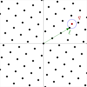
Let \(L\) be a lattice with some basis \(B \in \mathbb{R}^{n \times m}\) and \(\|\cdot\|\) some norm. Let \(\lambda (L)\) be the length of the shortest nonzero vector in \(L\). The task of finding \(l \in L\) such that \(\|l\| = \lambda(L)\), i.e. finding any shortest vector of \(L\), is called \(\textbf{shortest vector problem (SVP)}\).

1.4 Closest vector problem

Let \(L\) be a lattice with some basis \(B \in \mathbb{R}^{n \times m}\) and \(\|\cdot\|\) some norm. Given \(q \in \mathbb{R}^n\), the task of finding \(l \in L\) such that \(\|l-q\|\) is minimal, i.e. finding the lattice vector \(l\) closest to a given arbitrary vector, is called \(\textbf{closest vector problem (CVP)}\).

2. LWE fundamentals

2.1 Learning with errors

Let \(\mathbb{Z}_q = \mathbb{Z}/q \mathbb{Z}\) be the ring of integers modulo \(q\), i.e., the set of integers smaller than \(q\) with the operations \(+\) and \(\cdot\) modulo \(q\). As in high school, we can naturally form a linear equation system

\( \begin{align*} A\cdot s = b \quad \text{,} \end{align*} \)

where \(A\in \mathbb{Z}_q^{n\times m}, s\in \mathbb{Z}_q^m, b \in \mathbb{Z}_q^{n}\). For example, consider the following system:

\( \begin{align*} A = \begin{pmatrix} 10 & 3 & 5 & 1 \\ 4 & 1 & 1 & 2 \\ \vdots &\vdots & \vdots& \vdots\\ 3 & 1 & 1 & 5 \\ \end{pmatrix}, \quad b = \begin{pmatrix} 10 \\ 3 \\ \vdots \\ 8 \end{pmatrix} \end{align*} \)

Then, the associated equations look like

\( \begin{align*} 10\cdot s_1 + 3\cdot s_2 + 5\cdot s_3 + 1\cdot s_4 &= 10\\ 4\cdot s_1 + 1\cdot s_2 + 1\cdot s_3 + 2\cdot s_4 &= 3\\ \vdots\\ 3\cdot s_1 + 1\cdot s_2 + 1\cdot s_3 + 5\cdot s_4 &= 8 \end{align*} \)

Solving this equation system can be efficiently realized using the Gaussian algorithm. However, adding even only small error values \(e\in \mathbb{Z}_q^n\) to the equation system yields

\( \begin{align*} A\cdot s + e = b \quad \text{,} \end{align*} \)

which renders solving the equation system and retrieving the solution vector \(s\) surprisingly hard. This fact is founded in the relation to the hard lattice problems described above, which is presented in a nutshell below.

2.2 Decisional LWE

The LWE problem can also be rephrased as a decision problem, usually abbreviated \(\textbf{dLWE}\). Given an LWE sample \((A, b)\) as defined above (\(s\) and \(e\) are kept secret), the task is to guess whether the values of \(b\) have been calculated as \(A \cdot s + e\) with small error values \(e\), or whether they have been chosen arbitrarily. Both variants are equivalently hard. The reduction from LWE to dLWE has been proven by Regev [Reg09, Lemma 4.2], the inverse reduction from dLWE to LWE is trivial.

2.3 Linking LWE to computational lattice problems

Consider an LWE problem of the form

\( \begin{align*} A\cdot s + e = b \quad \text{,} \end{align*} \)

where \(A\in \mathbb{Z}_q^{n\times m}, b \in \mathbb{Z}_q^{n}\) and small vectors \(s\in \mathbb{Z}_q^m, e \in \mathbb{Z}_q^{n}\). It is straightforward to solve a concrete LWE instance by solving the closest vector problem. Observe that the closest vector to \(b\) is almost always the lattice vector \(A \cdot s\) with distance \(e\).

To give an intuition of the relationship between learning with errors and the shortest vector problem, consider the lattice

\( \begin{align*} L = \{x \in \mathbb{Z}^{m+n+1} \mid (A \mid\mid I_n \mid\mid (-b)) \cdot x = 0 \mod q\} \quad \text{,} \end{align*} \)

where the '\(\mid \mid\)' operator denotes concatenation and \(I_n\) denotes the \(n \times n\) identity matrix. It can be observed that the column vector \((s, e, 1)\) is an element of \(L\) by verifying that

\( \begin{align*} \begin{pmatrix} A & I_n & -b \end{pmatrix} \cdot \begin{pmatrix} s \\ e \\ 1 \end{pmatrix} = A \cdot s + e -b = b-b = 0 \ mod \ q \end{align*} \)

holds. It can be shown that the vector \((s, e, 1)\) is actually a shortest vector in \(L\) and therefore is an SVP solution for \(L\). This means, retrieving the vector \((s, e, 1)\) directly yields the secret \(s\) as well as the error vector \(e\) and therefore solves the LWE system.

2.4 LWE-based encryption schemes

This section aims to serve as a high-level introduction to LWE-based encryption schemes, so that their basic idea can be easily understood. The following simplified example will only be used to transmit a message consisting of a single bit, but it can be trivially extended to transmit a bitstring of any desired length.

Consider an LWE instance \(A \cdot s + e = b\), where \(A \in \mathbb{Z}_q^{n \times m}\) is chosen uniformly random and \(s\in \mathbb{Z}_q^m\) and \(e\in \mathbb{Z}_q^n\) are chosen from an error distribution, i.e. their values are rather small. Let's assume the values \(A\) and \(b\) are public while the corresponding values \(s\) and \(e\) are kept secret. The LWE problem then states that it is hard to calculate \(s\) or \(e\).

To build the actual encryption scheme, we will randomly sample the additional values \(r \in \mathbb{Z}_q^n\) as well as errors \(e_1 \in \mathbb{Z}_q^m\) and \(e_2 \in \mathbb{Z}_q\). With that, we construct the equation system

\( \begin{align*} u &= A^T \cdot r + e_1 ~~ \in \mathbb{Z}_q^m\\ v &= b^T \cdot r + e_2 ~~ \in \mathbb{Z}_q \quad \text{,} \end{align*} \)

which can be equivalently represented as

\( \begin{align*} \begin{pmatrix} u\\ v \end{pmatrix} &= \begin{pmatrix} A^T\\ b^T \end{pmatrix} r + \begin{pmatrix} e_1\\ e_2 \end{pmatrix} \end{align*} \)

in a compact form.

It is then easy to see that this is also another instance of the LWE problem. With knowledge of \((A, b, u, v)\) it is hard to calculate any of the other values. Furthermore, the decisional LWE problem states that it is even hard to differentiate between the values \(u, v\) calculated in the way described above and \(u, v'\) with some arbitrary value \(v'\). This is a core part of our encryption system.

For now, let us assume we would just send \((u, v)\) back to the recipient, who (knowing \(s\)) could then calculate the value \(s^T \cdot u = s^T \cdot (A^T \cdot r + e_1)\). Taking into account that the error values are relatively small, we observe that \(s^T \cdot u \approx s^T \cdot A^T \cdot r\), and also that \(v = b^T \cdot r + e_2 \approx b^T \cdot r \approx (A \cdot s)^T \cdot r = s^T \cdot A^T \cdot r\). Thus, neglecting the error values, we get that \(s^T \cdot u \approx v\).

This means we have found a way to indirectly transmit about the same value in two separate ways and we have done so unnoticeable by a third person: Without knowledge of \(s\) it cannot be deduced how close exactly these values are to each other (dLWE assumption).

The trick is to hide the message in one of these values. When the message is \(0\), we will just transmit \(v' = v\). However, in case it is \(1\), we will transmit \(v' = v + q/2\) (remember that we are operating on \(\mathbb{Z}_q\), so this is the value "opposite'' to \(0\)). The receiver can then calculate \(\mu = v' - s^T \cdot u\). If \(\mu\) is close to zero (mod \(q\)), the message was \(0\), if it is closer to \(q/2\), the message was \(1\).

Let us summarize the process more formally. Let \(\text{round}_n(\cdot)\) denote rounding to the nearest multiple of \(n\). For a one-bit message encoded as \(\mu \in \{0, \lfloor q/2 \rfloor\}\), the ciphertext is \((u,v')\) with

\( \begin{align*} u &= A^T \cdot r + e_1 \\ v' &= b^T \cdot r + e_2 + \mu \quad \text{,} \end{align*} \)

from which the receiver can calculate

\( \begin{align*} \phantom{{}={}} \text{round}&_{\lfloor q/2 \rfloor}( v' - s^T \cdot u ) \\ &= \text{round}_{\lfloor q/2 \rfloor}( b^T r + e_2 + \mu - s^T(A^T r + e_1) ) \\ &= \text{round}_{\lfloor q/2 \rfloor}( (As + e)^T r + e_2 + \mu - s^T A^T r - s^T e_1 ) \\ &= \text{round}_{\lfloor q/2 \rfloor}( (As)^T r + e^T r + e_2 + \mu - (As)^T r - s^T e_1 ) \\ &= \text{round}_{\lfloor q/2 \rfloor}( \mu + e^T r + e_2 - s^T e_1 ) \\ &= \mu. \end{align*} \)

For the last equality to hold (and thus, the decryption to succeed), we need the overall effect of the error term \((e^T r + e_2 - s^T e_1)\) to stay below \(q/4\). In practice, relevant schemes use an error distribution and a modulus \(q\) where this is not always the case in order to have reasonable ciphertext sizes. The failure probability is extremely small (see table 3.1), so it is usually negligible in practice. However, care must be taken that attackers cannot learn anything about the secret key by intentionally crafting ciphertexts that cause decryption failures.

2.5 Flavors of LWE: Ring-LWE and Module-LWE

The sample cryptosystem described above can be trivially extended to encapsulate bitstrings of a fixed length \(\ell\) by running the same protocol \(\ell\) times in parallel. In contrast to the flavors described below, this approach is called \(\textbf{Plain LWE}\). Because of its simplicity it is considered to have the least potential for attacks. However, this is paid for by communication costs about 15 times higher than with Ring-LWE or Module-LWE. A production-ready scheme that uses Plain LWE is Frodo [BCD+16]. Because of the relatively bad performance it is not among the NIST standardization finalists (but included as an alternate candidate) and thus not included in this report. Other variants of LWE can be created by exchanging the underlying algebraic structure. Various flavors have been researched, we will detail the relevant ones in the following.

\(\textbf{Ring-LWE}\) was first proposed by Vadim Lyubashevsky, Chris Peikert and Oded Regev in 2010 [LPR10]. Calculations take place in a polynomial ring \(R_q := \mathbb{Z}_q[x] / f(x)\) for some polynomial \(f(x)\). Therefore, polynomial multiplication is used instead of matrix multiplication.

\(\textbf{Module-LWE}\) is a variant that further improves Ring-LWE and was proposed by Adeline Langlois and Damien Stehlé in 2012 [LS12]. It uses the exact same structure as the sample system detailed above, but the scalars are replaced by ring elements of \(R_q\) as defined in the previous paragraph. Consequently, vectors become elements of so-called modules, which are a generalization of vector spaces over rings, hence the name.

Most early practical implementations of LWE-based cryptography, such as the NewHope scheme [ADPS15], use Ring-LWE. However, it was shown that Ring-LWE possibly provides more attack surface, so that a Ring-LWE scheme is at most as secure as an equally-parameterized Module-LWE scheme [PP19]. For that reason, NIST has decided not to consider Ring-LWE schemes in the third round.

Table 2.1: Comparison of algebraic structures used in LWE variants
	Plain LWE	Ring-LWE	Module-LWE

\(\mathbf{A}\)	\(\mathbb{Z}_q^{n \times m}\)	\(\mathbb{Z}_q[x]/f\)	\(( \mathbb{Z}_q[x]/f)^{n \times m}\)
\(\mathbf{\cdot}\)	matrix mult.	polynomial mult.	matrix mult.
\(\mathbf{s}\)	\(\mathbb{Z}_q^m\)	\(\mathbb{Z}_q[x]/f\)	\(( \mathbb{Z}_q[x]/f)^m\)
\(\mathbf{b,e}\)	\(\mathbb{Z}_q^n\)	\(\mathbb{Z}_q[x]/f\)	\(( \mathbb{Z}_q[x]/f)^n\)

3. Kyber

Kyber [ABD+21] is a CCA-secure KEM derived from a CPA-secure public-key encryption (PKE) scheme based on Module-LWE. For \(n, q \in \mathbb{N}\), the underlying ring is \(R_q = \mathbb{Z}_q[X] \ / \ (X^n+1)\), i.e. the ring of polynomials up to degree \(n-1\) with coefficients in \(\mathbb{Z}_q\). The corresponding module is \(R_q^k\) with rank \(k \in \mathbb{N}\).

The following primitives are required: a noise space \(B\), where sampling a value from \(B\) yields a random small integer value in the range \(\{-4,..., 4\}\). Additionally, for the KEM construction, secure hash functions \(H_1,H_2\) and a secure key derivation function \(KDF\) are required.

Internally, the plaintext encrypted by Kyber is a ring element \(r \in R_q\). Therefore, the input bitstring \(m \in \{0,1\}^{256}\) is converted to a ring element \(r = toRing(m)\), i.e. a polynomial, as follows:

\( \begin{align*} \begin{pmatrix} 0 \\ 0 \\ 1 \\ \vdots \\ 0 \\ 1 \end{pmatrix} \xrightarrow{toRing} \begin{pmatrix} 0 \\ 0 \\ \lceil \frac{q}{2} \rceil \\ \vdots \\ 0 \\ \lceil \frac{q}{2} \rceil \end{pmatrix} \iff 0 + 0 \cdot x + \frac{q}{2} \cdot x^2 + ... + 0 \cdot x^{n-2} + \frac{q}{2} \cdot x^{n-1} \end{align*} \)

It can already be observed that even after having added a vector with small coefficients the original polynomial can easily be reconstructed. The reverse operation \(fromRing\) reconstructs a bitstring from a given ring element through coefficient-wise division by \(\frac{q}{2}\) and subsequent rounding. (The Kyber specification introduces encoding and compression functions, which we have simplified to the \(toRing\) and \(fromRing\) functions to increase readability and understanding.)

Analogously to the general LWE-based encryption scheme described in section 2.4, the Kyber key generation instantiates a particular LWE problem \(As + e = b\) by generating coefficients \(A\) for the linear equation system and sampling a solution vector \(s\) as well as an error vector \(e\).

Algorithm 1. Kyber PKE Key Generation: keyGen
Input: none
1. Generate \( A \in R_q^{k \times k} \)
2. Sample \( s \in R_q^k \) with coefficients from \( B \)
3. Sample \( e \in R_q^k \) with coefficients from \( B \)
4. Calculate \( b = As + e \)

Output: public key \( pk = (A, b) \), secret key \( s \)

The solution vector \(s\) functions as the secret key while \(A\) and the vector \(b = As+e\) are used as the public key. Calculating \(s\) from the public key would be identical to solving an instance of the LWE problem.

The Kyber PKE encryption looks similar to the LWE-based encryption scheme introduced in section 2.4 expanded to a Module-LWE setting.

Algorithm 2. Kyber PKE Encryption: enc
Input: public key \( pk = (A, b) \), message \( m \in \{0,1\}^{256}\)
1. Sample \( r \in R_q^k \) with coefficients from \( B \)
2. Sample \( e_1 \in R_q^k\) with coefficients from \( B \)
3. Sample \( e_2 \in R_q \) with coefficients from \( B \)
4. Calculate \( u = A^Tr+e_1 \)
5. Calculate \( v = b^Tr + e_2 + toRing(m)\)

Output: ciphertext \( c=(u,v)\)

With knowledge of the secret value \(s\), the reconstruction of the message \(m\) is possible through the corresponding Kyber PKE decryption routine.

Algorithm 3. Kyber PKE Decryption: dec
Input: secret key \( s \), ciphertext \( c = (u,v)\)
1. Calculate \( m^* = v-s^Tu \)

Output: message \( m = fromRing(m^*)\)

Applying the operation \(fromRing(m^*)\) reconstructs the original \(m\) with very high probability. Indeed, the Kyber encryption scheme is a probabilistic algorithm returning the original message \(m\) with very high probability (see table 3.1) for concrete failure probability values), depending on the amount of noise within the sampled vectors.

To construct a CCA-secure KEM from the given PKE, a variant of the Fujisaki-Okamoto transformation (FO-transformation) is used. Fujisaki and Okamoto [FO13] presented the first generic transformation from asymmetric and symmetric encryption schemes to a secure hybrid encryption scheme. Later, Hofheinz, Hövelmanns and Kiltz [HHK17] extended the work of Fujisaki and Okamoto and presented a generic transformation toolkit including a transformation of a PKE scheme into a secure KEM.

Algorithm 4. Kyber KEM Key Generation
Input: none
1. Generate \( \sigma \in \{0,1\}^{256} \)
2. Generate \( (pk, s) = PKE.keyGen()\)

Output: public key \( pk \), secret key \( sk = (s,\sigma) \)

In the KEM encapsulation, observe that the value \(r\) is used in the underlying PKE as a seed for the generation of the otherwise random values during encryption. Although a deterministic public key encryption algorithm is usually not desirable, for a KEM the receiver needs to be able to repeat the encryption procedure in the same way as the sender. We denote the deterministic version of the encryption routine with given seed \(r\) by \(PKE.enc_r(pk,m)\). Furthermore, the message \(m\) is hashed before being fed to the PKE encryption routine.

Algorithm 5. Kyber KEM Encapsulation
Input: public key \( pk \)
1. Generate message \( m \in \{0,1\}^{256}\)
2. Calculate \( (K',r) = H_1(H_2(m) \mid\mid H_2(pk))\)
3. Calculate \( c = PKE.enc_r(pk, H_2(m)) \)
4. Calculate \( K = KDF(K' \mid\mid H_2(c))\)

Output: encapsulation \( c \), shared secret \( K \)

The decapsulation routine calculates the required values analogously to the encapsulation routine.

Algorithm 6. Kyber KEM Decapsulation
Input: public key \( pk \), secret key \( sk = (s,\sigma) \), encapsulation \( c \)
1. Calculate \( H_m = PKE.dec(s, c)\)
2. Calculate \( (K',r') = H_1(H_m \mid\mid H_2(pk))\)
3. Calculate \( c' = PKE.enc_{r'}(pk, H_m) \)
4. If \( c = c' \text{, set } K = KDF(K' \mid\mid H_2(c))\)
5. If \( c \neq c' \text{, set } K = KDF(\sigma \mid\mid H_2(c))\)

Output: shared secret \( K\)

To gain some intuition of how ciphertext validation in Kyber works, have a look at the decryption process as described in detail in section 2.4. In the Kyber PKE scheme, the message \(m\) is embedded within the difference of the vectors \(v\) and \(s^Tu\), i.e.

\begin{align*} v - s^T \cdot u = toRing(m) + (e^Tr + e_2 - s^T e_1) \quad \text{,} \end{align*}

where \(e, e_1, e_2\) are random error vectors. There are a lot of different combinations of values of these error terms that all correspond to the same \(m\). In the KEM, however, the randomness becomes deterministic by deriving it from a chosen \(r\), so there is a unique set of values \((e, e_1, e_2)\) for each \(m\). This property establishes the required CCA-security of the KEM. When an adversary sends a random ciphertext to the decapsulation routine, it will always decipher to a message \(m\), but the probability that the adversary has chosen the specific ciphertext (generated by the correct "random" terms) corresponding to \(m\) is negligible.

Table 3.1: Kyber parameter sets with corresponding decryption failure probability \(\delta\)
	\(n\)	\(k\)	\(q\)	\(\delta\)

Kyber512	256	2	3329	2^-139
Kyber768	256	3	3329	2^-164
Kyber1024	256	4	3329	2^-174

4. Dilithium

For \(n, q \in \mathbb{N}\), the underlying ring is \(R_q = \mathbb{Z}_q[X] \ / \ (X^n+1)\), i.e. the ring of polynomials up to degree \(n-1\) with coefficients in \(\mathbb{Z}_q\). The corresponding module is \(R_q^l\) with rank \(l \in \mathbb{N}\). Additionally, Dilithium requires a secure hash function \(H\).

The key generation is almost identical to Kyber's key generation. An LWE instance is generated, i.e. a matrix \(A \in R_q^{k \times l}\) with \(k \in \mathbb{N}\), a secret vector \(s \in R_q^l\) and an error term \(e \in R_q^k\). As usual, \(A\) and \(b\) are public while \(s\) is kept private.

Algorithm 7. Dilithium Key Generation: keyGen
Input: none
1. Generate \( A \in R_q^{k \times l}\)
2. Sample \( s \in R_q^l\) with small coefficients
3. Sample \( e \in R_q^k \) with small coefficients
4. Calculate \( b = As + e\)

Output: public key \( pk = (A, b)\), secret key \( s \)

Dilithium's signing process is probabilistic. In the first step a random vector \(y \in R_q^l\) is sampled. As we will see in the verification process, to achieve correctness we will use the rounded version of \(Ay\) by means of a function \(round()\). This function takes a given vector of polynomials and rounds each coefficient of every polynomial. The signature is formed by calculating a pair \((z,c)\), where \(c\) is formed by hashing the message \(m\) and the value \(round(Ay)\). The hash function \(H\) maps an input to a polynomial with coefficients in \(\{-1, 0, 1\}\).

Due to the fact that \(z\) depending on the secret key \(s\) potentially leads to serious security issues, \(z\) is not output directly. Instead, in order to remove the statistical dependencies between \(z\) and \(s\), Dilithium follows a so-called \(\textit{rejection sampling}\) approach. For the details of rejection sampling we refer to [Lyu12] and [BG14]. In case \(z\) is rendered invalid ('rejected'), the algorithm restarts from step \(1\).

Algorithm 8. Dilithium Signature generation
Input: public key \( pk = (A, b) \), secret key \( s\), message \( m \in \{0,1\}^{\star}\)
Until \( z\) is valid:
1. Sample \( y \in R_q^l\) with small coefficients
2. Calculate \( w = round(Ay) \)
3. Calculate \( c = H(m \mid\mid w)\)
4. Calculate \( z = y + cs\)

Output: signature \( \sigma = (z,c)\)

Given a correct signature \(\sigma\), it is possible to recover \(w\) by the following calculation:

\begin{align*} round(Az-bc) &= round(A(y+cs)-(As+e)c) \\ &= round(Ay + Acs - Acs - ce) \\ &= round(Ay - ce) \\ &= w \end{align*}

To indeed recover \(w\), the last step requires \(round(Ay-ce) = round(Ay)\). Since \(c\) and \(e\) both have small coefficients, their product \(ce\) does not influence the outcome of the rounding. In order to verify the signature, we can use a recovered \(w'\) to recalculate \(c' = H(m \mid\mid w')\) and compare it to the provided signature value \(c\). Observe, that if \(z\) has not been calculated by using the secret key \(s\), i.e. by \(z = y + cs\), the terms \(Acs\) would not cancel in the equation above leading to an incorrect \(w' \neq w\). Hence, the value \(c'\) would be incorrect as well leading to a rejection of the provided signature.

Algorithm 9. Dilithium Verification
Input: public key \( pk = (A, b) \), message \( m \in \{0,1\}^{\star}\), signature \( \sigma = (z,c)\)
1. Calculate \( w' = round(Az-bc)\)
2. Calculate \( c' = H(m \mid\mid w')\)

Output: valid if \( c = c'\), else invalid

Table 4.1: Dilithium parameter sets for NIST security levels 2,3,5 with corresponding expected number of needed repetitions \(\#reps\) of signature generation
	\(n\)	\((k,l)\)	\(q\)	\(\#reps\)

Dilithium 2	256	(4,4)	8380417	4.25
Dilithium 3	256	(6,5)	8380417	5.1
Dilithium 5	256	(8,7)	8380417	3.85

This blog post is part of our blog series »Post-Quantum Cryptography in Practice« and an excerpt of the study »A Mathematical Perspective on Post-Quantum Cryptography«, which gives an overview of the round-three finalist of NIST’s post-quantum cryptography standardization process. It introduces the mathematical fundamentals of the lattice-based key encapsulation mechanisms (KEMs) CRYSTALS-Kyber, NTRU and SABER; the code-based KEM Classic McEliece; the lattice-based signature schemes CRYSTALS-Dilithium and FALCON; and the multivariate-based signature scheme Rainbow.

5. Bibliography

[ABD+21]
Roberto Avanzi, Joppe Bos, Léo Ducas, Eike Kiltz, Tancr`ede Lepoint, Vadim Lyubashevsky, John M. Schanck, Peter Schwabe, Gregor Seiler, and Damien Stehlé. CRYSTALSKYBER: Algorithm specifications and supporting documentation, Jan. 2021.

[ADPS15]
Erdem Alkim, Léo Ducas, Thomas Pöppelmann, and Peter Schwabe. Post-quantum key exchange – a new hope. Cryptology ePrint Archive, Report 2015/1092, 2015. https://ia.cr/2015/1092.

[BCD+16]
Joppe Bos, Craig Costello, Leo Ducas, Ilya Mironov, Michael Naehrig, Valeria Nikolaenko, Ananth Raghunathan, and Douglas Stebila. Frodo: Take off the ring! practical, quantumsecure key exchange from lwe. pages 1006–1018, 10 2016.

[BDK+20]
Shi Bai, Léo Ducas, Eike Kiltz, Tancrede Lepoint, Vadim Lyubashevsky, Peter Schwabe, Gregor Seiler, and Damien Stehlé. CRYSTALS-Dilithium: Algorithm specifications and supporting documentation, Oct. 2020.

[BG14]
Shi Bai and Steven D. Galbraith. An improved compression technique for signatures based on learning with errors. In Josh Benaloh, editor, Topics in Cryptology – CT-RSA 2014, pages 28–47, Cham, 2014. Springer International Publishing.

[CJL+16]
Lily Chen, Stephen Jordan, Yi-Kai Liu, Dustin Moody, Rene Peralta, Ray Perlner, and Daniel Smith-Tone. Report on Post-Quantum Cryptography. Technical Report NIST Internal or Interagency Report (NISTIR) 8105, National Institute of Standards and Technology,
April 2016.

[FO13]
Eiichiro Fujisaki and Tatsuaki Okamoto. Secure Integration of Asymmetric and Symmetric Encryption Schemes. Journal of Cryptology, 26(1):80–101, January 2013.

[HHK17]
Dennis Hofheinz, Kathrin Hövelmanns, and Eike Kiltz. A Modular Analysis of the Fujisaki-Okamoto Transformation. In Yael Kalai and Leonid Reyzin, editors, Theory of Cryptography, volume 10677, pages 341–371. Springer International Publishing, Cham, 2017. Series Title: Lecture Notes in Computer Science.

[LPR10]
Vadim Lyubashevsky, Chris Peikert, and Oded Regev. On ideal lattices and learning with errors over rings. In Henri Gilbert, editor, Advances in Cryptology – EUROCRYPT 2010, pages 1–23, Berlin, Heidelberg, 2010. Springer Berlin Heidelberg.

[LS12]
Adeline Langlois and Damien Stehle. Worst-case to average-case reductions for module lattices. Cryptology ePrint Archive, Report 2012/090, 2012. https://ia.cr/2012/090.

[Lyu12]
Vadim Lyubashevsky. Lattice signatures without trapdoors. In David Pointcheval and Patrick Schaumont, editors, EUROCRYPT 2012 – 31st Annual International Conference on the Theory and Applications of Cryptographic Techniques, Cambridge, UK, April 15-19, 2012., volume 7237 of Lecture Notes in Computer Science, pages 738–755, Cambridge, United Kingdom, April 2012. Springer.

[PP19]
Chris Peikert and Zachary Pepin. Algebraically structured lwe, revisited. Cryptology ePrint Archive, Report 2019/878, 2019. https://ia.cr/2019/878.

[Reg09]
Oded Regev. On lattices, learning with errors, random linear codes, and cryptography. Journal of the ACM, 56(6):34:1–34:40, September 2009.

Authors

Maximilian Richter

Maximilian Richter is an IT security researcher and passionate about mathematical aspects of cryptography. After studying both mathematics and computer science and several years of practical experience as a working student with focus on risk and threat modeling, design of secure system architectures and cryptographic software development, he does research at Fraunhofer AISEC in the areas of post-quantum cryptography, quantum cryptanalysis, secure systems and digital identities since 2020.

Contact: maximilian.richter@aisec.fraunhofer.de

Jasper Seidensticker

Jasper Seidensticker is an M.Sc. student of mathematics at FU Berlin and works at Fraunhofer AISEC as a student researcher since 2021. His main fields of research are cryptography and cryptanalysis with a focus on post-quantum-cryptography, especially lattice-based primitives.

Contact: jasper.seidensticker@aisec.fraunhofer.de

Magdalena Bertram

Magdalena Bertram has been a student researcher at Fraunhofer AISEC in the Secure Software Engineering department since 2020. She completed her Bachelor’s degree in mathematics and is currently writing her Master’s thesis in computer science in the field of lattice-based signature schemes. Her areas of focus include post-quantum cryptography, cryptanalysis, and digital identities.

Contact: magdalena.bertram@aisec.fraunhofer.de

A (somewhat) gentle introduction to lattice-based post-quantum cryptography

Table of contents